This article is an introduction to the basics of window functions in SQL. First, in the introduction, I will explain what is a window function and what it does. Then, I will show you how to write window functions. Finally, I will go through the different types of window functions we can use. At the end of the article, I will link to some practical examples of how we can use those functions. More examples will be added later as I write more articles on the topic.
Introduction
A window function performs calculations against a partition of the data. The two main characteristics of window functions are: - They don't collapse rows of a group - They can run calculations on a set of rows related to the current row.
Let's see what it means.
- Window functions don't collapse rows of a group.
The difference with aggregation functions using the
GROUP BYclause is that the result is not grouped into single rows. Instead, the resultset contains every row of each group. To illustrate, we'll write queries that sum the salaries of each department of a company.
Aggregation functions return a single result per group, hiding the rows of each group.
 department_name  |   sum
------------------+----------
 Accounting       | 20300.00
 Administration   |  4400.00
 Executive        | 58000.00
 Finance          | 51600.00
 Human Resources  |  6500.00
 IT               | 28800.00
 Marketing        | 19000.00
 Public Relations | 10000.00
 Purchasing       | 24900.00
 Sales            | 57700.00
 Shipping         | 41200.00
(11 rows)
When using a window function, all the rows of each group are returned.
 department_name  |   sum
------------------+----------
 Accounting       | 20300.00
 Accounting       | 20300.00
 Administration   |  4400.00
 Executive        | 58000.00
[...]
 Shipping         | 41200.00
 Shipping         | 41200.00
 Shipping         | 41200.00
(40 rows)
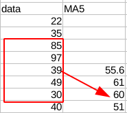
- Window functions can run calculations on a set of rows related to the current row.
Window functions can run their calculation on a window that 'slides' along the dataset. It can include a number of rows before and/or after the current row.
A common example of such operation is how we calculate a moving average. For example, a 5 periods moving average will only include the last five rows:
In the example below, \(60 = \frac{85+97+39+49+30}{5}\).
Syntax
A window function call always contains an OVER clause. The OVER clause is what defines the window partitions.
function(expression) OVER([PARTITION BY expression_list]
                          [ORDER BY order_list]
                          [ROWS frame_clause])
The OVER() clause
The OVER() clause is where the partitionning of the window function is set. It contains three clauses:
- PARTITION BY
- ORDER BY
- ROWS or RANGE
PARTITION BY
Splits the table into partitions based on a column's unique values.
Let's have a look at salaries:
If I write the following query,
SELECT MAX(salary) FROM salaries;
I get a unique row with the highest of all salaries:
   max
----------
 24000.00
(1 row)
If I want to get the maximum salary for each department, I can use the PARTITION BY department clause:
SELECT
    employee
    , department
    , salary
    , MAX(salary) OVER(PARTITION BY department) AS department_max
FROM
    salaries
;
     employee      |    department    |  salary  | department_max
-------------------+------------------+----------+----------------
 William Gietz     | Accounting       |  8300.00 |       12000.00
 Shelley Higgins   | Accounting       | 12000.00 |       12000.00
 Jennifer Whalen   | Administration   |  4400.00 |        4400.00
 Lex De Haan       | Executive        | 17000.00 |       24000.00
 Steven King       | Executive        | 24000.00 |       24000.00
 Neena Kochhar     | Executive        | 17000.00 |       24000.00
...
For each row, I get the maximum salary for that department. For example, we can see that Shelley Higgins has the highest salary in the Accounting department.
ORDER BY
Specifies the order of rows in a partition. From the previous example, we can order the rows by employee:
SELECT
    employee
    , department
    , salary
    , MAX(salary) OVER(PARTITION BY department ORDER BY employee) AS department_max
FROM
    salaries
;
     employee      |    department    |  salary  | department_max
-------------------+------------------+----------+----------------
 Shelley Higgins   | Accounting       | 12000.00 |       12000.00
 William Gietz     | Accounting       |  8300.00 |       12000.00
 Jennifer Whalen   | Administration   |  4400.00 |        4400.00
 Lex De Haan       | Executive        | 17000.00 |       17000.00
 Neena Kochhar     | Executive        | 17000.00 |       17000.00
 Steven King       | Executive        | 24000.00 |       24000.00
 Daniel Faviet     | Finance          |  9000.00 |        9000.00
 Ismael Sciarra    | Finance          |  7700.00 |        9000.00
 John Chen         | Finance          |  8200.00 |        9000.00
 Jose Manuel Urman | Finance          |  7800.00 |        9000.00
We now have the departments that are grouped together and all employees of a department are sorted alphabetically.
ROWS or RANGE
The last clause defines the frame. This is a subset of rows against which the function is run.
It can either specify where the frame starts only:
{RANGE | ROWS} frame_start
Or it can specify where the frame starts and where it ends:
{RANGE | ROWS} BETWEEN frame_start AND frame_end
frame_start is one of the following options:
- N PRECEDING: N rows before the current row.
- UNBOUNDED PRECEDING: all the rows preceding the current row.
- CURRENT ROW
frame_end is one of the following options:
- CURRENT ROW
- N FOLLOWING: N rows after the current row.
- UNBOUNDED FOLLOWING: all the rows following the current row.
Setting up the frame start only:
SELECT
    payment_date
    , amount
    , SUM(amount) OVER(ROWS UNBOUNDED PRECEDING) AS unbounded
    , SUM(amount) OVER(ROWS 3 PRECEDING) AS nrows
    , SUM(amount) OVER(ROWS CURRENT ROW) AS current_row
FROM
    daily_sales
;
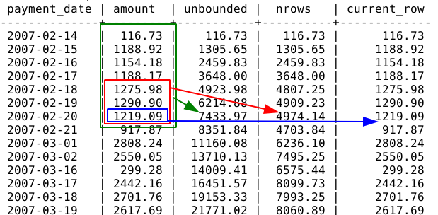
Let's look at some example using BETWEEN ... AND ...:
SELECT
    payment_date
    , amount
    , SUM(amount) OVER(ROWS BETWEEN UNBOUNDED PRECEDING AND 2 FOLLOWING) AS all_til_next_two
    , SUM(amount) OVER(ROWS BETWEEN 3 PRECEDING AND 2 FOLLOWING) AS six_rows
    , SUM(amount) OVER(ROWS BETWEEN CURRENT ROW AND UNBOUNDED FOLLOWING) AS all_following
FROM
    daily_sales
;
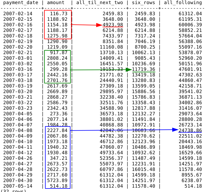
The BETWEEN UNBOUNDED PRECEDING AND 2 FOLLOWING clause will sum all the amounts from the beginning (UNBOUNDED PRECEDING) until two rows after the current row (2 FOLLOWING) as shown by the red frame.
The BETWEEN 3 PRECEDING AND 2 FOLLOWING clause will sum all the amounts from three rows before the current row (3 PRECEDING) until two rows after the current row (2 FOLLOWING) as shown by the green frame.
Finally, the BETWEEN CURRENT ROW AND UNBOUNDED FOLLOWING clause will sum all the amounts from the current row to the last row (UNBOUNDED FOLLOWING) as shown by the blue frame.
What is the difference between ROWS and RANGE To check the difference between ROWS and RANGE, I am going to write a query that sums the salaries using each of the frames keywords:
SELECT
    salary
    , SUM(salary) OVER(ORDER BY salary ROWS CURRENT ROW) AS rows
    , SUM(salary) OVER(ORDER BY salary RANGE CURRENT ROW) AS range
FROM
    salaries
;
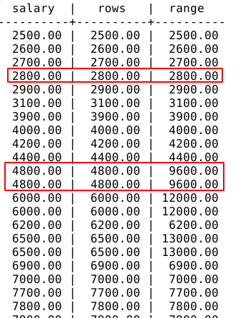
We can see there's a difference when there are duplicate values. RANGE returns all rows with the same value as a unique current row. In our example, there are two employees with a salary of 4800. When using ROWS, the sum returns 4800 for each of the rows. When using RANGE, the sum returns 9600 (4800 + 4800) on both rows.
Window functions types
Value window functions
The value window functions return the value of a column or expression at a specified row of a resultset.
FIRST_VALUE()
The FIRST_VALUE() function returns the first value in a sorted partition.
syntax:
FIRST_VALUE(expression) OVER()
Example:
Let's write a query that gives us the name of the employee who has the lowest salary of each department. We'll build the window function as follow:
- partition the data by department: PARTITION BY department.
- order the salaries to get the lowest one in the first row of the partition: ORDER BY salary.
- get the name of the employee in the first row of the partition: FIRST_VALUE(employee).
The final query will look like this:
    SELECT
        employee_id
        , employee
        , department
        , salary
        , FIRST_VALUE(employee) OVER(PARTITION BY department ORDER BY salary)
    FROM
        salaries
    ;
 employee_id |     employee      |    department    |  salary  |    first_value
-------------+-------------------+------------------+----------+-------------------
         206 | William Gietz     | Accounting       |  8300.00 | William Gietz
         205 | Shelley Higgins   | Accounting       | 12000.00 | William Gietz
         200 | Jennifer Whalen   | Administration   |  4400.00 | Jennifer Whalen
         102 | Lex De Haan       | Executive        | 17000.00 | Lex De Haan
         101 | Neena Kochhar     | Executive        | 17000.00 | Lex De Haan
         100 | Steven King       | Executive        | 24000.00 | Lex De Haan
         113 | Luis Popp         | Finance          |  6900.00 | Luis Popp
         111 | Ismael Sciarra    | Finance          |  7700.00 | Luis Popp
         112 | Jose Manuel Urman | Finance          |  7800.00 | Luis Popp
...
LAST_VALUE()
The LAST_VALUE() function returns the value of the last row of the partition.
Unlike the FIRST_VALUE() function, it requires that the frame is specified in the OVER() clause.
Syntax:
LAST_VALUE(expression) OVER()
Example:
We can use the same example we used for the first_value() function. This time, we want to see who has the highest salary in each department:
- partition the data by department: PARTITION BY department.
- order the salaries to get the highest one in the last row of the partition: ORDER BY salary.
- get the name of the employee in the last row of the partition: LAST_VALUE(employee).
SELECT
    employee_id
    , employee
    , department
    , salary
    , LAST_VALUE(employee) OVER(PARTITION BY department ORDER BY salary ROWS BETWEEN UNBOUNDED PRECEDING AND UNBOUNDED FOLLOWING)
FROM
    salaries
;
 employee_id |     employee      |    department    |  salary  |    last_value
-------------+-------------------+------------------+----------+-------------------
         206 | William Gietz     | Accounting       |  8300.00 | Shelley Higgins
         205 | Shelley Higgins   | Accounting       | 12000.00 | Shelley Higgins
         200 | Jennifer Whalen   | Administration   |  4400.00 | Jennifer Whalen
         102 | Lex De Haan       | Executive        | 17000.00 | Steven King
         101 | Neena Kochhar     | Executive        | 17000.00 | Steven King
         100 | Steven King       | Executive        | 24000.00 | Steven King
         113 | Luis Popp         | Finance          |  6900.00 | Nancy Greenberg
         111 | Ismael Sciarra    | Finance          |  7700.00 | Nancy Greenberg
         112 | Jose Manuel Urman | Finance          |  7800.00 | Nancy Greenberg
         110 | John Chen         | Finance          |  8200.00 | Nancy Greenberg
         109 | Daniel Faviet     | Finance          |  9000.00 | Nancy Greenberg
         108 | Nancy Greenberg   | Finance          | 12000.00 | Nancy Greenberg
...
LAG()
The LAG() funciton accesses the row that is n rows before the current row. We can also set a default value that will be returned when the row does not exist.
Syntax:
LAG(expression, offset, default) OVER()
where offset is the number of rows before the current row from which we want the data.
Example:
We can use the LAG() function to compare daily sales with the previous week sales. To do so, we:
- order the sales by date: ORDER BY payment_date.
- get the amount from 7 days before: LAG(amount, 7).
- we can add a default value for the first 7 rows: LAG(amount, 7, 0::numeric).
The final query looks like this:
WITH daily_sales AS(
    SELECT
        payment_date::date
        , SUM(amount) as amount
    FROM
        payment
    GROUP BY
        payment_date::date
)
SELECT
    payment_date
    , amount
    , LAG(amount, 7, 0::numeric) OVER(ORDER BY payment_date) AS previous_week_amount
FROM
    daily_sales
;
 payment_date | amount  | previous_week_amount
--------------+---------+----------------------
 2007-02-14   |  116.73 |                    0
 2007-02-15   | 1188.92 |                    0
 2007-02-16   | 1154.18 |                    0
 2007-02-17   | 1188.17 |                    0
 2007-02-18   | 1275.98 |                    0
 2007-02-19   | 1290.90 |                    0
 2007-02-20   | 1219.09 |                    0
 2007-02-21   |  917.87 |               116.73
 2007-03-01   | 2808.24 |              1188.92
 2007-03-02   | 2550.05 |              1154.18
 2007-03-16   |  299.28 |              1188.17
 2007-03-17   | 2442.16 |              1275.98
 ...
LEAD()
The LEAD() function is similar to the LAG() but it returns the value of the nth row following the current row.
Syntax:
LEAD(expression, offset, default) OVER()
Example:
We can write a query that gives us the sales of the next week:
- order the sales by date: ORDER BY payment_date.
- get the amount 7 days after the date of the current row: LEAD(amount, 7).
WITH daily_sales AS(
    SELECT
        payment_date::date
        , SUM(amount) as amount
    FROM
        payment
    GROUP BY
        payment_date::date
)
SELECT
    payment_date
    , amount
    , LEAD(amount, 7) OVER(ORDER BY payment_date) AS next_week_amount
FROM
    daily_sales
;
 payment_date | amount  | next_week_amount
--------------+---------+------------------
 2007-02-14   |  116.73 |           917.87
 2007-02-15   | 1188.92 |          2808.24
 2007-02-16   | 1154.18 |          2550.05
 2007-02-17   | 1188.17 |           299.28
 2007-02-18   | 1275.98 |          2442.16
 2007-02-19   | 1290.90 |          2701.76
 2007-02-20   | 1219.09 |          2617.69
 2007-02-21   |  917.87 |          2669.89
 2007-03-01   | 2808.24 |          2868.27
 2007-03-02   | 2550.05 |          2586.79
 2007-03-16   |  299.28 |          2342.43
 2007-03-17   | 2442.16 |           273.36
 2007-03-18   | 2701.76 |          2077.14
 2007-03-19   | 2617.69 |          1984.28
 2007-03-20   | 2669.89 |          2227.84
 ...
NTH_VALUE()
The NTH_VALUE() returns the value from the Nth row of a partition.
Syntax:
NTH_VALUE(expression, offset) OVER()
- expression: the target column or an expression.
- offset: integer that determines the row number relative to the first row of the partition.
Example:
For this example, I'll simply write a query that gives the third salary from the lowest one for each department:
- Group the salaries per department: PARTITION BY department.
- Order the salaries: ORDER BY salary.
- Get the third salary: NTH_VALUE(salary, 3).
SELECT
    employee
    , department
    , salary
    , NTH_VALUE(salary, 3) OVER(PARTITION BY department ORDER BY salary) AS third_salary
FROM
    salaries
;
     employee      |    department    |  salary  | third_salary
-------------------+------------------+----------+--------------
 William Gietz     | Accounting       |  8300.00 |
 Shelley Higgins   | Accounting       | 12000.00 |
 Jennifer Whalen   | Administration   |  4400.00 |
 Lex De Haan       | Executive        | 17000.00 |
 Neena Kochhar     | Executive        | 17000.00 |
 Steven King       | Executive        | 24000.00 |     24000.00
[...]
 Irene Mikkilineni | Shipping         |  2700.00 |
 Britney Everett   | Shipping         |  3900.00 |
 Sarah Bell        | Shipping         |  4000.00 |      4000.00
 Shanta Vollman    | Shipping         |  6500.00 |      4000.00
 Payam Kaufling    | Shipping         |  7900.00 |      4000.00
 Matthew Weiss     | Shipping         |  8000.00 |      4000.00
 Adam Fripp        | Shipping         |  8200.00 |      4000.00
(40 rows)
When the total number of rows of a partition is less than the offset, the NTH_VALUE() function returns a Null value.
Ranking window functions
ROW_NUMBER()
the ROW_NUMBER() function returns the number of the current row within its partition.
Syntax:
ROW_NUMBER() OVER()
Example:
SELECT
        employee
        , department
        , salary
        , ROW_NUMBER() OVER(ORDER BY department,salary) AS row_number
        , ROW_NUMBER() OVER(PARTITION BY department ORDER BY department,salary) AS row_number_per_department
FROM
        salaries
;
     employee      |    department    |  salary  | row_number | row_number_per_department
-------------------+------------------+----------+------------+---------------------------
 William Gietz     | Accounting       |  8300.00 |          1 |                         1
 Shelley Higgins   | Accounting       | 12000.00 |          2 |                         2
 Jennifer Whalen   | Administration   |  4400.00 |          3 |                         1
 Lex De Haan       | Executive        | 17000.00 |          4 |                         1
 Neena Kochhar     | Executive        | 17000.00 |          5 |                         2
 Steven King       | Executive        | 24000.00 |          6 |                         3
[...]
 Shanta Vollman    | Shipping         |  6500.00 |         37 |                         4
 Payam Kaufling    | Shipping         |  7900.00 |         38 |                         5
 Mattlhew Weiss     | Shipping         |  8000.00 |         39 |                         6
 Adam Fripp        | Shipping         |  8200.00 |         40 |                         7
(40 rows)
CUME_DIST()
The CUME_DIST() function calculate the cumulative distribution of a value. This is the number of rows with values less or equal to the value of the current row divided by the total number of rows.
Syntax:
CUME_DIST() OVER()
Example:
SELECT
    employee
    , department
    , salary
    , CUME_DIST() OVER(ORDER BY salary)
FROM
    salaries
;
     employee      |    department    |  salary  | cume_dist
-------------------+------------------+----------+-----------
 Karen Colmenares  | Purchasing       |  2500.00 |     0.025
 Guy Himuro        | Purchasing       |  2600.00 |      0.05
 Irene Mikkilineni | Shipping         |  2700.00 |     0.075
 Sigal Tobias      | Purchasing       |  2800.00 |       0.1
 Shelli Baida      | Purchasing       |  2900.00 |     0.125
 Alexander Khoo    | Purchasing       |  3100.00 |      0.15
 Britney Everett   | Shipping         |  3900.00 |     0.175
 Sarah Bell        | Shipping         |  4000.00 |       0.2
 Diana Lorentz     | IT               |  4200.00 |     0.225
 ...
In the example above, we can see that 20% of employees have a salary that is less or equal to 4000.
RANK and DENSE_RANK()
The RANK() and the DENSE_RANK() functions return the rank of the current row. The difference is that the DENSE_RANK() function result has no gap while the RANK() function will skip ranks when rows have the same values.
Syntax:
- DENSE_RANK()
DENSE_RANK() OVER()
- RANK()
RANK() OVER()
Example:
SELECT
    employee
    , department
    , salary
    , RANK() OVER(ORDER BY salary)
    , DENSE_RANK() OVER(ORDER BY salary)
FROM
    salaries
;
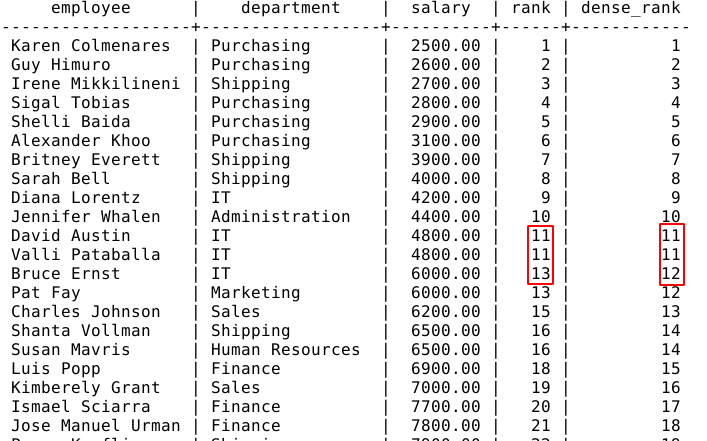
In the example above, we can see that there are two employees with a salary of 4,800. Both of them get the rank 11 in the rank and the dense_rank columns.
However, the following employee's rank is 13 in the rank column and 12 in the dense_rank columns.
The DENSE_RANK() function didn't skip any value. The RANK() returns the actual row number of the first row with a given value.
PERCENT_RANK()
The PERCENT_RANK() function returns the relative rank of the current row:
The values range from 0 to 1.
Syntax:
PERCENT_RANK() OVER()
Example:
SELECT
    employee
    , department
    , salary
    , PERCENT_RANK() OVER(ORDER BY department,salary) AS pct_rank
    , PERCENT_RANK() OVER(PARTITION BY department ORDER BY department,salary) AS department_pct_rank
FROM
    salaries
;
     employee      |    department    |  salary  |      pct_rank       | department_pct_rank
-------------------+------------------+----------+---------------------+---------------------
 William Gietz     | Accounting       |  8300.00 |                   0 |                   0
 Shelley Higgins   | Accounting       | 12000.00 | 0.02564102564102564 |                   1
 Jennifer Whalen   | Administration   |  4400.00 | 0.05128205128205128 |                   0
 Lex De Haan       | Executive        | 17000.00 | 0.07692307692307693 |                   0
 Neena Kochhar     | Executive        | 17000.00 | 0.07692307692307693 |                   0
 Steven King       | Executive        | 24000.00 |  0.1282051282051282 |                   1
[...]
 Irene Mikkilineni | Shipping         |  2700.00 |  0.8461538461538461 |                   0
 Britney Everett   | Shipping         |  3900.00 |  0.8717948717948718 | 0.16666666666666666
 Sarah Bell        | Shipping         |  4000.00 |  0.8974358974358975 |  0.3333333333333333
 Shanta Vollman    | Shipping         |  6500.00 |  0.9230769230769231 |                 0.5
 Payam Kaufling    | Shipping         |  7900.00 |  0.9487179487179487 |  0.6666666666666666
 Matthew Weiss     | Shipping         |  8000.00 |  0.9743589743589743 |  0.8333333333333334
 Adam Fripp        | Shipping         |  8200.00 |                   1 |                   1
(40 rows)
NTILE()
The NTILE() function breaks a resultset into a specified number of buckets. All the buckets have about the same number of rows.
Syntax:
NTILE(number_buckets) OVER()
Example:
SELECT
        employee
        , department
        , salary
        , NTILE(4) OVER(ORDER BY salary) AS four_buckets
        , NTILE(10) OVER(ORDER BY salary) AS ten_buckets
FROM
        salaries
;
     employee      |    department    |  salary  | four_buckets | ten_buckets
-------------------+------------------+----------+--------------+-------------
 Karen Colmenares  | Purchasing       |  2500.00 |            1 |           1
 Guy Himuro        | Purchasing       |  2600.00 |            1 |           1
 Irene Mikkilineni | Shipping         |  2700.00 |            1 |           1
 Sigal Tobias      | Purchasing       |  2800.00 |            1 |           1
 Shelli Baida      | Purchasing       |  2900.00 |            1 |           2
 Alexander Khoo    | Purchasing       |  3100.00 |            1 |           2
 Britney Everett   | Shipping         |  3900.00 |            1 |           2
 Sarah Bell        | Shipping         |  4000.00 |            1 |           2
 Diana Lorentz     | IT               |  4200.00 |            1 |           3
 Jennifer Whalen   | Administration   |  4400.00 |            1 |           3
 David Austin      | IT               |  4800.00 |            2 |           3
 Valli Pataballa   | IT               |  4800.00 |            2 |           3
[...]
 Karen Partners    | Sales            | 13500.00 |            4 |           9
 John Russell      | Sales            | 14000.00 |            4 |          10
 Neena Kochhar     | Executive        | 17000.00 |            4 |          10
 Lex De Haan       | Executive        | 17000.00 |            4 |          10
 Steven King       | Executive        | 24000.00 |            4 |          10
(40 rows)
We have 40 employees. The NTILE(4) columns returns four buckets numbered 1 to 4 and containing ten employees each. The NTILE(10) column returns 10 buckets numbered 1 to 10 and containing four employees each.
Aggregate window functions
Those are the usual aggregate functions we would use with a GROUP BY clause:
- AVG(): average.
- SUM(): sum.
- MIN(): minimum value.
- MAX(): maximum value.
- COUNT(): rows count.
SELECT
    employee
    , department
    , salary
    , AVG(salary) OVER(PARTITION BY department) AS dpt_avg_salary
    , SUM(salary) OVER(PARTITION BY department) AS dpt_total_salary
    , MIN(salary) OVER(PARTITION BY department) AS dpt_min_salary
    , MAX(salary) OVER(PARTITION BY department) AS dpt_max_salary
    , COUNT(*) OVER(PARTITION BY department) AS dpt_count
FROM
    salaries
ORDER BY
    department
    ,salary
;
     employee      |    department    |  salary  |     dpt_avg_salary     | dpt_total_salary | dpt_min_salary | dpt_max_salary | dpt_count
-------------------+------------------+----------+------------------------+------------------+----------------+----------------+-----------
 William Gietz     | Accounting       |  8300.00 | 10150.0000000000000000 |         20300.00 |        8300.00 |       12000.00 |         2
 Shelley Higgins   | Accounting       | 12000.00 | 10150.0000000000000000 |         20300.00 |        8300.00 |       12000.00 |         2
 Jennifer Whalen   | Administration   |  4400.00 |  4400.0000000000000000 |          4400.00 |        4400.00 |        4400.00 |         1
 Lex De Haan       | Executive        | 17000.00 |     19333.333333333333 |         58000.00 |       17000.00 |       24000.00 |         3
 Neena Kochhar     | Executive        | 17000.00 |     19333.333333333333 |         58000.00 |       17000.00 |       24000.00 |         3
 Steven King       | Executive        | 24000.00 |     19333.333333333333 |         58000.00 |       17000.00 |       24000.00 |         3
 Luis Popp         | Finance          |  6900.00 |  8600.0000000000000000 |         51600.00 |        6900.00 |       12000.00 |         6
 Ismael Sciarra    | Finance          |  7700.00 |  8600.0000000000000000 |         51600.00 |        6900.00 |       12000.00 |         6
 Jose Manuel Urman | Finance          |  7800.00 |  8600.0000000000000000 |         51600.00 |        6900.00 |       12000.00 |         6
 John Chen         | Finance          |  8200.00 |  8600.0000000000000000 |         51600.00 |        6900.00 |       12000.00 |         6
 Daniel Faviet     | Finance          |  9000.00 |  8600.0000000000000000 |         51600.00 |        6900.00 |       12000.00 |         6
 Nancy Greenberg   | Finance          | 12000.00 |  8600.0000000000000000 |         51600.00 |        6900.00 |       12000.00 |         6
       6
Examples
How to calculate a moving average in SQL