About RFM segmentation
Customer segmentation is important for multiple reasons. We get a deeper knowledge of our customers and can tailor targeted marketing campaigns.
The RFM method was introduced by Bult and Wansbeek in 1995 and has been successfully used by marketers since.
It analyzes customers' behavior on three parameters:
Recency: How recent is the last purchase of the customer.
Frequency: How often the customer makes a purchase.
Monetary: How much money does the customer spends.
The advantages of RFM is that it is easy to implement and it can be used for different types of business. It helps craft better marketing campaigns and improves CRM and customer's loyalty.
The disadvantages are that it may not apply in industries where customers are usually one time buyers. It is based on historical data and won't give much insight about prospects.
In this post, I will show how we can use RFM segmentation with Python.
Methodology
To get the RFM score of a customer, we need to first calculate the R, F and M scores on a scale from 1 (worst) to 5 (best).
- calculate Recency = number of days since last purchase
- calculate Freqency = number of purchases during the studied period (usually one year)
- calculate Monetary = total amount of purchases made during the studied period
- find quintiles for each of these dimensions
- give a grade to each dimension depending in which quintiles it stands
- combine R, F and M scores to get the RFM score
- map RF scores to segments
For this example, I will use the Online Retail dataset available on the UCI Machine Learning Repository.
Calculcate the RFM score
Prepare the data
import pandas as pd
from datetime import timedelta
import matplotlib.pyplot as plt
I create a dataframe with the sales data
sales = pd.read_excel('online-retail.xlsx')
sales.columns
Index(['InvoiceNo', 'StockCode', 'Description', 'Quantity', 'InvoiceDate',
        'UnitPrice', 'CustomerID', 'Country'],
      dtype='object')
print('{:,} rows; {:,} columns'.format(sales.shape[0], sales.shape[1]))
541,909 rows; 8 columns
print('{:,} invoices don\'t have a customer id'.format(sales[sales.CustomerID.isnull()].shape[0]))
135,080 invoices don't have a customer id
I am going to drop those lines as they will not help in our analysis of customers.
sales.dropna(subset=['CustomerID'], inplace=True)
What is the time frame of the data?
print('Orders from {} to {}'.format(sales['InvoiceDate'].min(),
                                    sales['InvoiceDate'].max()))
Orders from 2010-12-01 08:26:00 to 2011-12-09 12:50:00
We have about one year of sales data (from December 2010 to December 2011). This is the period usually used for RFM analysis. I'll set the period of the study to 365 days to get exactly one year.
I calculate the total price of each line.
sales['Price'] = sales['Quantity'] * sales['UnitPrice']
Next, I control whether there's only one row per invoice.
sales['InvoiceNo'].value_counts().head()
576339    542
579196    533
580727    529
578270    442
573576    435
Name: InvoiceNo, dtype: int64
Invoices can have multiple rows (one row per item). However, I am interested in how many times did a customer purchase, not how many items did he buy. I want to count orders rather than items.
I create an order dataframe that will aggregate our sales at the order level.
orders = sales.groupby(['InvoiceNo', 'InvoiceDate', 'CustomerID']).agg({'Price': lambda x: x.sum()}).reset_index()
orders.head()
| InvoiceNo | InvoiceDate | CustomerID | Price | |
|---|---|---|---|---|
| 0 | 536365 | 2010-12-01 08:26:00 | 17850.0 | 139.12 |
| 1 | 536366 | 2010-12-01 08:28:00 | 17850.0 | 22.20 |
| 2 | 536367 | 2010-12-01 08:34:00 | 13047.0 | 278.73 |
| 3 | 536368 | 2010-12-01 08:34:00 | 13047.0 | 70.05 |
| 4 | 536369 | 2010-12-01 08:35:00 | 13047.0 | 17.85 |
Finally, I am going to simulate an analysis I am doing in real time by setting the NOW date at one day after the last purchase. This date will be used as a reference to calculate the Recency score.
NOW = orders['InvoiceDate'].max() + timedelta(days=1)
NOW
Timestamp('2011-12-10 12:50:00')
I am going to study the data over a period of one year. I set a period variable to 365 (days).
You can change this value depending on your needs. It will depend on the industry and the expected behavior of customers but one year is a commonly used value in RFM segmentation.
period = 365
Calculate the Recency, Frequency and Monetary Value of each customers
To make things easier, I am going to add a column with the number of days between the purchase and now. To find the Recency values, I will just have to find the minimum of this column for each customer.
orders['DaysSinceOrder'] = orders['InvoiceDate'].apply(lambda x: (NOW - x).days)
The scores are calculated for each customer. I need a dataframe with one row per customer. The scores will be stored in columns.
aggr = {
    'DaysSinceOrder': lambda x: x.min(),  # the number of days since last order (Recency)
    'InvoiceDate': lambda x: len([d for d in x if d >= NOW - timedelta(days=period)]), # the total number of orders in the last period (Frequency)
}
rfm = orders.groupby('CustomerID').agg(aggr).reset_index()
rfm.rename(columns={'DaysSinceOrder': 'Recency', 'InvoiceDate': 'Frequency'}, inplace=True)
rfm.head()
| CustomerID | Recency | Frequency | |
|---|---|---|---|
| 0 | 12346.0 | 326 | 2 |
| 1 | 12347.0 | 2 | 6 |
| 2 | 12348.0 | 75 | 4 |
| 3 | 12349.0 | 19 | 1 |
| 4 | 12350.0 | 310 | 1 |
I have the Recency and Frequency data. I need to add the Monetary value of each customer by adding sales over the last year.
rfm['Monetary'] = rfm['CustomerID'].apply(lambda x: orders[(orders['CustomerID'] == x) & \
                                                           (orders['InvoiceDate'] >= NOW - timedelta(days=period))]\
                                                           ['Price'].sum())
rfm.head()
| CustomerID | Recency | Frequency | Monetary | |
|---|---|---|---|---|
| 0 | 12346.0 | 326 | 2 | 0.00 |
| 1 | 12347.0 | 2 | 6 | 3598.21 |
| 2 | 12348.0 | 75 | 4 | 1797.24 |
| 3 | 12349.0 | 19 | 1 | 1757.55 |
| 4 | 12350.0 | 310 | 1 | 334.40 |
Calculate the R, F and M scores
At this point, I have the values for Recency, Frequency and Monetary parameters. Each customer will get a note between 1 and 5 for each parameter.
We can do this by setting ranges based on expected behavior. For example, to rate Recency, we could use this scale:
1: 0-30 days
2: 31-60 days
3: 61-90 days
4: 91-180 days
5: 181-365 days
We could also use quintiles. Each quintiles contains 20% of the population. Using quintiles is more flexible as the ranges will adapt to the data and would work across different industries or if there's any change in expected customer behavior.
I am going to use the quintiles method. First, I get the quintiles for each parameter.
quintiles = rfm[['Recency', 'Frequency', 'Monetary']].quantile([.2, .4, .6, .8]).to_dict()
quintiles
{'Frequency': {0.2: 1.0, 0.4: 2.0, 0.6: 3.0, 0.8: 6.0},
  'Monetary': {0.2: 215.89800000000002,
  0.4: 440.432,
  0.6: 876.3679999999999,
  0.8: 1909.6580000000006},
  'Recency': {0.2: 11.0, 0.4: 32.0, 0.6: 71.0, 0.8: 178.80000000000018}}
Then I write methods to assign ranks from 1 to 5. A smaller Recency value is better whereas higher Frequency and Monetary values are better. I need to write two separate methods.
def r_score(x):
    if x <= quintiles['Recency'][.2]:
        return 5
    elif x <= quintiles['Recency'][.4]:
        return 4
    elif x <= quintiles['Recency'][.6]:
        return 3
    elif x <= quintiles['Recency'][.8]:
        return 2
    else:
        return 1

def fm_score(x, c):
    if x <= quintiles[c][.2]:
        return 1
    elif x <= quintiles[c][.4]:
        return 2
    elif x <= quintiles[c][.6]:
        return 3
    elif x <= quintiles[c][.8]:
        return 4
    else:
        return 5
I am now ready to get the R, F and M scores of each customer.
rfm['R'] = rfm['Recency'].apply(lambda x: r_score(x))
rfm['F'] = rfm['Frequency'].apply(lambda x: fm_score(x, 'Frequency'))
rfm['M'] = rfm['Monetary'].apply(lambda x: fm_score(x, 'Monetary'))
Get customers segments from RFM score
Finally, I combine the R, F and M scores into a RFM Score.
rfm['RFM Score'] = rfm['R'].map(str) + rfm['F'].map(str) + rfm['M'].map(str)
rfm.head()
| CustomerID | Recency | Frequency | Monetary | R | F | M | RFM Score | |
|---|---|---|---|---|---|---|---|---|
| 0 | 12346.0 | 326 | 2 | 0.00 | 1 | 2 | 1 | 121 |
| 1 | 12347.0 | 2 | 6 | 3598.21 | 5 | 4 | 5 | 545 |
| 2 | 12348.0 | 75 | 4 | 1797.24 | 2 | 4 | 4 | 244 |
| 3 | 12349.0 | 19 | 1 | 1757.55 | 4 | 1 | 4 | 414 |
| 4 | 12350.0 | 310 | 1 | 334.40 | 1 | 1 | 2 | 112 |
The RFM scores give us 5\(^3\) = 125 segments. Which is not easy to work with.
I am going to work with 11 segments based on the R and F scores. Here is the description of the segments:
| Segment | Description |
|---|---|
| Champions | Bought recently, buy often and spend the most |
| Loyal Customers | Buy on a regular basis. Responsive to promotions. |
| Potential Loyalist | Recent customers with average frequency. |
| Recent Customers | Bought most recently, but not often. |
| Promising | Recent shoppers, but haven’t spent much. |
| Customers Needing Attention | Above average recency, frequency and monetary values. May not have bought very recently though. |
| About To Sleep | Below average recency and frequency. Will lose them if not reactivated. |
| At Risk | Purchased often but a long time ago. Need to bring them back! |
| Can’t Lose Them | Used to purchase frequently but haven’t returned for a long time. |
| Hibernating | Last purchase was long back and low number of orders. May be lost. |
The resulting matrix look like this:
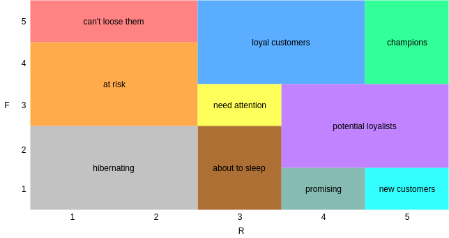
segt_map = {
    r'[1-2][1-2]': 'hibernating',
    r'[1-2][3-4]': 'at risk',
    r'[1-2]5': 'can\'t loose',
    r'3[1-2]': 'about to sleep',
    r'33': 'need attention',
    r'[3-4][4-5]': 'loyal customers',
    r'41': 'promising',
    r'51': 'new customers',
    r'[4-5][2-3]': 'potential loyalists',
    r'5[4-5]': 'champions'
}

rfm['Segment'] = rfm['R'].map(str) + rfm['F'].map(str)
rfm['Segment'] = rfm['Segment'].replace(segt_map, regex=True)
rfm.head()
| CustomerID | Recency | Frequency | Monetary | R | F | M | RFM Score | Segment | |
|---|---|---|---|---|---|---|---|---|---|
| 0 | 12346.0 | 326 | 2 | 0.00 | 1 | 2 | 1 | 121 | hibernating |
| 1 | 12347.0 | 2 | 6 | 3598.21 | 5 | 4 | 5 | 545 | champions |
| 2 | 12348.0 | 75 | 4 | 1797.24 | 2 | 4 | 4 | 244 | at risk |
| 3 | 12349.0 | 19 | 1 | 1757.55 | 4 | 1 | 4 | 414 | promising |
| 4 | 12350.0 | 310 | 1 | 334.40 | 1 | 1 | 2 | 112 | hibernating |
Visualize our customers segments
Now that we have our scores, we can do some data visualization to get a better idea of our customers portfolio. First, let see at the distribution of R, F and M.
# plot the distribution of customers over R and F
fig, axes = plt.subplots(nrows=1, ncols=2, figsize=(10, 4))

for i, p in enumerate(['R', 'F']):
    parameters = {'R':'Recency', 'F':'Frequency'}
    y = rfm[p].value_counts().sort_index()
    x = y.index
    ax = axes[i]
    bars = ax.bar(x, y, color='silver')
    ax.set_frame_on(False)
    ax.tick_params(left=False, labelleft=False, bottom=False)
    ax.set_title('Distribution of {}'.format(parameters[p]),
                fontsize=14)
    for bar in bars:
        value = bar.get_height()
        if value == y.max():
            bar.set_color('firebrick')
        ax.text(bar.get_x() + bar.get_width() / 2,
                value - 5,
                '{}\n({}%)'.format(int(value), int(value * 100 / y.sum())),
               ha='center',
               va='top',
               color='w')

plt.show()

# plot the distribution of M for RF score
fig, axes = plt.subplots(nrows=5, ncols=5,
                         sharex=False, sharey=True,
                         figsize=(10, 10))

r_range = range(1, 6)
f_range = range(1, 6)
for r in r_range:
    for f in f_range:
        y = rfm[(rfm['R'] == r) & (rfm['F'] == f)]['M'].value_counts().sort_index()
        x = y.index
        ax = axes[r - 1, f - 1]
        bars = ax.bar(x, y, color='silver')
        if r == 5:
            if f == 3:
                ax.set_xlabel('{}\nF'.format(f), va='top')
            else:
                ax.set_xlabel('{}\n'.format(f), va='top')
        if f == 1:
            if r == 3:
                ax.set_ylabel('R\n{}'.format(r))
            else:
                ax.set_ylabel(r)
        ax.set_frame_on(False)
        ax.tick_params(left=False, labelleft=False, bottom=False)
        ax.set_xticks(x)
        ax.set_xticklabels(x, fontsize=8)

        for bar in bars:
            value = bar.get_height()
            if value == y.max():
                bar.set_color('firebrick')
            ax.text(bar.get_x() + bar.get_width() / 2,
                    value,
                    int(value),
                    ha='center',
                    va='bottom',
                    color='k')
fig.suptitle('Distribution of M for each F and R',
             fontsize=14)
plt.tight_layout()
plt.show()
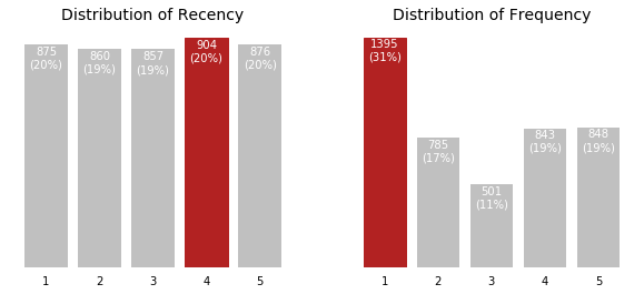
We can see that if recency seems evenly distributed, almost half of the customers don't purchase very often (48% of customers have a frequency of 1 or 2).
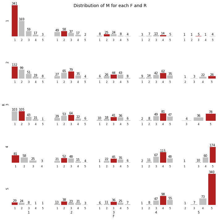
When looking at the monetary value, we see that the customers spending the most are those with the highest activity (R and F of 4-5). We have very few large orders (high monetary value but low frequency).
Let's look at the distribution of our segments.
I am not going to use a treemap like the segments matrix shown above to visualize the distribution of segments. Bar charts are a better fit for comparing quantities.
# count the number of customers in each segment
segments_counts = rfm['Segment'].value_counts().sort_values(ascending=True)

fig, ax = plt.subplots()

bars = ax.barh(range(len(segments_counts)),
              segments_counts,
              color='silver')
ax.set_frame_on(False)
ax.tick_params(left=False,
               bottom=False,
               labelbottom=False)
ax.set_yticks(range(len(segments_counts)))
ax.set_yticklabels(segments_counts.index)

for i, bar in enumerate(bars):
        value = bar.get_width()
        if segments_counts.index[i] in ['champions', 'loyal customers']:
            bar.set_color('firebrick')
        ax.text(value,
                bar.get_y() + bar.get_height()/2,
                '{:,} ({:}%)'.format(int(value),
                                   int(value*100/segments_counts.sum())),
                va='center',
                ha='left'
               )

plt.show()
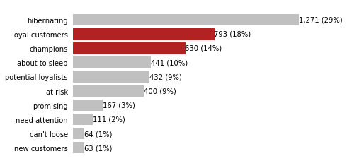
We have a lot of customers who don't buy frequently from us (29% are hibernating). However, 32% of our customers are either champions or loyal customers.
Further analysis can be done that integrate the Monetary parameters.
With customers assigned to segments and some statistics on the composition of our customers portfolio, we can work on targeted marketing campaigns to retain customers that are at risk, improve sales to customers with some potential and reward the best customers.