Machine learning practitioners rely on ensembles to improve the performance of their model. One of the methods used for ensembling multiple models is to calculate the weighted average of their predictions. The problem that rises is how to find the weights that will give us the best ensemble. In this post, I will explain how to optimize those weights using scipy. But before starting, I want to give credit to Tilii from who I got this method that he used in this kernel.
For this example, I will work on a regression problem using the boston dataset available in scikit-learn.
First, I load the data:
import numpy as np
from sklearn.datasets import load_boston

boston = load_boston()
X = boston.data
y = boston.target
features = boston.feature_names
print(features)
['CRIM' 'ZN' 'INDUS' 'CHAS' 'NOX' 'RM' 'AGE' 'DIS' 'RAD' 'TAX' 'PTRATIO' 'B' 'LSTAT']
I'll work with only one feature for easy visualization.
I'll use RM (Avg number of rooms)
X = X[:,5].reshape(-1, 1)
Then I split the dataset into a train and test sets. I'll use the test set to evaluate my final model.
from sklearn.model_selection import train_test_split

X_train, X_test, y_train, y_test = train_test_split(X, y, test_size=.2, random_state=0)
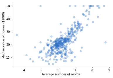
Let's have a quick pick at the data.
import matplotlib.pyplot as plt

fig = plt.figure()
ax = fig.add_subplot(111)

ax.scatter(X_train, y_train, facecolor=None, edgecolor='royalblue', alpha=.3)

ax.spines['top'].set_visible(False)
ax.spines['right'].set_visible(False)

ax.set_xlabel('Average number of rooms')
ax.set_ylabel('Median value of homes ($1000)')

plt.show()
I am going to work with two models only. I'll ensemble a linear model and a tree based model.
I choose a simple linear regression and a single decision tree to get weaker base models.
from sklearn.linear_model import LinearRegression
from sklearn.tree import DecisionTreeRegressor

model_1 = LinearRegression()
model_2 = DecisionTreeRegressor(max_depth=3, random_state=0)
Then, I need to generate out-of-fold (oof) predictions on the train set.
What are out-of-fold predictions?
We fit our model on a train set then we make predictions on a test set using the trained model. I am going to do the same for my ensemble. Here to fit the model is to find the best weights to calculate the average of the predictions from the base models. So to 'fit' my ensemble I need predictions made on the training set but I can't make predictions using data the model has already seen in the training phase. So for each base model, I need to train on a part of the training set and make predictions on another part. This is what we do in cross-validation.
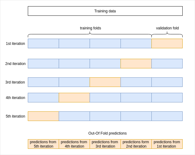
I am going to do a 5 folds cross validation. For each iteration, I will:
- train the models on the train folds.
- get predictions on the validation fold.
- store the predictions in an array.
At the end of cross validation, I will have an array for each model with predictions made on the training set. I will use those predictions as features to build my ensemble.
from sklearn.model_selection import KFold
from sklearn.metrics import mean_squared_error

kf = KFold(n_splits=5, random_state=0)

nrows_trn = X_train.shape[0]

# create an array for each model to store the oof predictions
mod1_oof_trn = np.empty(nrows_trn)
mod2_oof_trn = np.empty(nrows_trn)

# create arrays to store each iteration score
mod1_scores = np.empty(5)
mod2_scores = np.empty(5)

for k, (trn_idx, val_idx) in enumerate(kf.split(X_train, y_train)):
    # split the features and target into training and validation folds
    X_trn, X_val = X_train[trn_idx], X_train[val_idx]
    y_trn, y_val = y_train[trn_idx], y_train[val_idx]

    # train the first model on the train folds
    model_1.fit(X_trn, y_trn)
    # get the predictions on the validation fold
    # and save them in the array I created previously
    mod1_oof_trn[val_idx] = model_1.predict(X_val)
    # store the model score for this iteration
    mod1_scores[k] = mean_squared_error(y_val, mod1_oof_trn[val_idx])

    # do the same thing for the second model
    model_2.fit(X_trn, y_trn)
    mod2_oof_trn[val_idx] = model_2.predict(X_val)
    mod2_scores[k] = mean_squared_error(y_val, mod2_oof_trn[val_idx])
Now that I have the predictions on the train set, I can fit my models on all the train data to get predictions on the test set.
An alternative way would be to make predictions on the test set during cross validation and average the 5 predictions.
Create arrays to store the predictions:
nrows_tst = X_test.shape[0]
mod1_oof_tst = np.zeros(nrows_tst)
mod2_oof_tst = np.zeros(nrows_tst)
Then add those lines inside the CV script:
mod1_oof_tst += model_1.predict(X_test) / 5
mod2_oof_tst += model_2.predict(X_test) / 5
model_1.fit(X_train, y_train)
model_2.fit(X_train, y_train)

mod1_predictions = model_1.predict(X_test)
mod2_predictions = model_2.predict(X_test)
Let's have a look at how my models behave.
I am going to chart the boxplots of the CV scores and plot the regression lines of each model over the training data.
import matplotlib.gridspec as gridspec

print('Model 1 CV score: mean = {:.4f}; standard deviation = {:.4f}'.format(mod1_scores.mean(),
                                                                            mod1_scores.std()))
print('Model 2 CV score: mean = {:.4f}; standard deviation = {:.4f}'.format(mod2_scores.mean(),
                                                                            mod2_scores.std()))

fig = plt.figure(figsize=(10, 10))
G = gridspec.GridSpec(2, 2,
                     height_ratios=[1, 2])

ax1 = plt.subplot(G[0, :])
ax1.boxplot([mod1_scores, mod2_scores])
ax1.set_title('Models CV scores and regression lines', fontsize=16)
ax1.spines['bottom'].set_visible(False)
ax1.spines['top'].set_visible(False)
ax1.spines['right'].set_visible(False)
ax1.set_xticklabels(['Model 1', 'Model 2'], fontsize=12)
ax1.tick_params(bottom=False)

ax2 = plt.subplot(G[1, 0])

X_plot = np.arange(X_train.min(), X_train.max()).reshape(-1, 1)
y_plot = model_1.predict(X_plot)

ax2.scatter(X_train, y_train, facecolor=None, edgecolor='royalblue', alpha=.3)
ax2.plot(X_plot, y_plot, 'orange')
ax2.spines['top'].set_visible(False)
ax2.spines['right'].set_visible(False)
ax2.set_xlabel('Average Number of rooms')
ax2.set_ylabel('Median value of homes')

ax3 = plt.subplot(G[1, 1], sharey=ax2)

X_plot = np.arange(X_train.min(), X_train.max()).reshape(-1, 1)
y_plot = model_2.predict(X_plot)

ax3.scatter(X_train, y_train, facecolor=None, edgecolor='royalblue', alpha=.3)
ax3.plot(X_plot, y_plot, 'orange')
ax3.spines['top'].set_visible(False)
ax3.spines['right'].set_visible(False)
ax3.set_xlabel('Average number of rooms')

plt.tight_layout()
plt.show()
Model 1 CV score: mean = 43.2682; standard deviation = 8.6542
Model 2 CV score: mean = 39.3335; standard deviation = 10.3182
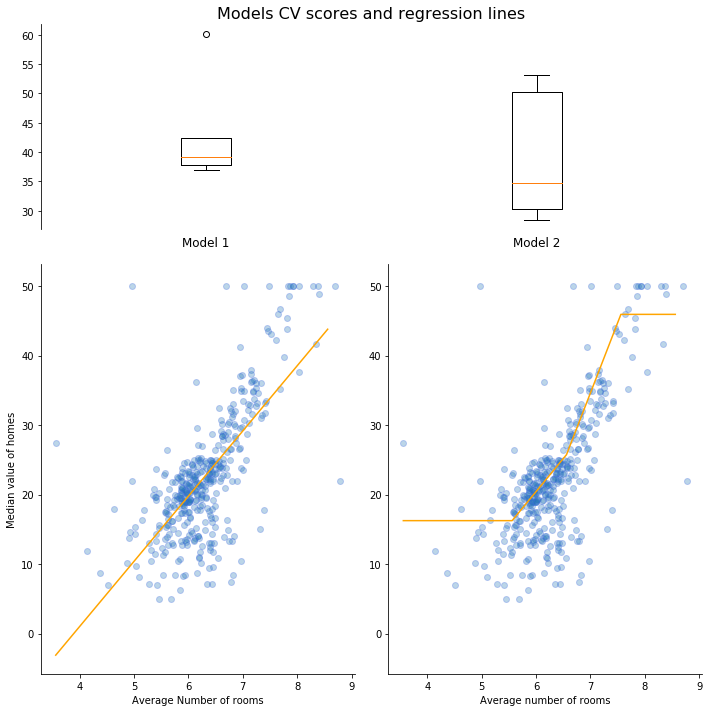
We can see that the first model (linear regression) has a higher error but lower variance than the second model (decision tree). Also, the regression lines are quite different except for a small segment where we have more data points.
This is a good configuration for ensembling. Ensembling models that are too similar gives a smaller improvement of the prediction performance.
I am now going to calculate the final predictions by calculating the weighted average of the predictions of those two models.
I will use scipy.optimize to find the best weights.
First, I blend the predictions in a matrix where each row is a sample and each column is the prediction from one of the models.
train_predictions = np.concatenate([mod1_oof_trn[:, None],
                                    mod2_oof_trn[:, None]], axis=1)
Then I need to define an objective function that I will have to minimize
def objective(weights):
    """ Calculate the score of a weighted average of predictions

    Parameters
    ----------
    weights: array
        the weights used to calculate the average of the ensembled
        predictions.

    Returns
    -------
    float
        The mean_squared_error score of the ensemble
    """

    y_ens = np.average(train_predictions, axis=1, weights=weights)
    return mean_squared_error(y_train, y_ens)
Finaly, I use the minimize function from scipy.optimize to find the weights that will give the lowest MSE score.
To avoid finding a local minima, I will run the optimization multiple time setting the initial weights at random.
from scipy.optimize import minimize

results_list = []    # a list to store the best score of each round
weights_list = []    # a list to store the best weights of each round

for k in range(100):
    # I randomly set the initial weights from which the algorithm will try searching a minima
    w0 = np.random.uniform(size=train_predictions.shape[1])

    # I define bounds, i.e. lower and upper values of weights.
    # I want the weights to be between 0 and 1.
    bounds = [(0,1)] * train_predictions.shape[1]

    # I set some constraints. Here, I want the sum of the weights to be equal to 1
    cons = [{'type': 'eq',
             'fun': lambda w: w.sum() - 1}]

    # I can now search for the best weights
    res = minimize(objective,
                   w0,
                   method='SLSQP',
                   bounds=bounds,
                   options={'disp':False, 'maxiter':10000},
                   constraints=cons)

    # I save the best score and the best weights of
    # this round in their respective lists
    results_list.append(res.fun)
    weights_list.append(res.x)

# After running all the rounds, I extract the best score
# and the corresponding weights
best_score = np.min(results_list)
best_weights = weights_list[results_list.index(best_score)]

print('\nOptimized weights:')
print('Model 1: {:.4f}'.format(best_weights[0]))
print('Model 2: {:.4f}'.format(best_weights[1]))
print('Best score: {:.4f}'.format(best_score))
Optimized weights:
Model 1: 0.3726
Model 2: 0.6274
Best score: 37.1407
Now, we can have a look at how our models perform on the test set.
I am going to look at the performance of the two base models, the unoptimized ensemble (average without weights) and the optimized ensemble.
# individual scores
print('Model 1 test score = {:.4f}'.format(mean_squared_error(y_test, mod1_predictions)))
print('Model 2 test score = {:.4f}'.format(mean_squared_error(y_test, mod2_predictions)))

# unoptimized ensemble
test_predictions = np.concatenate([mod1_predictions[:, None],
                                   mod2_predictions[:, None]], axis=1)
unoptimized_ensemble = np.average(test_predictions, axis=1)
print('Unoptimized ensemble test score: {:.4f}'.format(mean_squared_error(y_test,
                                                                          unoptimized_ensemble)))

# optimized ensemble
optimized_ensemble = np.average(test_predictions, axis=1, weights=best_weights)
print('Optimized ensemble test score: {:.4f}'.format(mean_squared_error(y_test,
                                                                        optimized_ensemble)))

fig = plt.figure(figsize=(10, 10))
ax = fig.add_subplot(111)
ax.scatter(X_test, y_test, color=None, edgecolor='b', alpha=.4)

X_plot = np.arange(X_test.min(), X_test.max() + 1).reshape(-1, 1)
line_1 = model_1.predict(X_plot)
line_2 = model_2.predict(X_plot)
blend = np.concatenate([line_1[:, None],
                        line_2[:, None]], axis=1)
line_ens = np.average(blend, axis=1, weights=w0)
line_opt = np.average(blend, axis=1, weights=best_weights)

ax.plot(X_plot, model_1.predict(X_plot), c='b', alpha=.7, label='model 1')
ax.plot(X_plot, model_2.predict(X_plot), c='r', alpha=.7, label='model 2')
ax.plot(X_plot, line_ens, c='orange', alpha=.7, label='unoptimized ensemble')
ax.plot(X_plot, line_opt, c='g', alpha=.7, label='optimized ensemble')

ax.spines['top'].set_visible(False)
ax.spines['right'].set_visible(False)

ax.legend()
ax.set_title('Comparison of regression lines of all models', fontsize=16)
ax.set_xlabel('Average number of rooms')
ax.set_ylabel('Median value of homes')
plt.show()
Model 1 test score = 46.9074
Model 2 test score = 40.2115
Unoptimized ensemble test score: 40.2323
Optimized ensemble test score: 39.5951
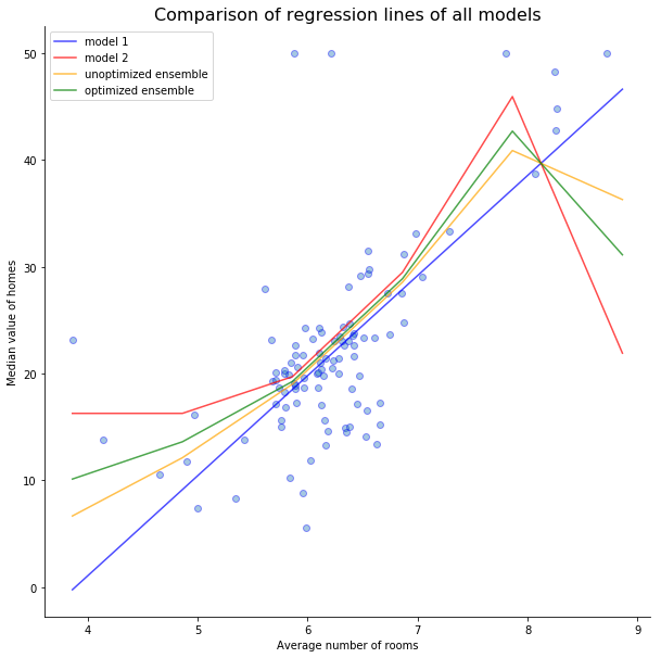
As we can see here, the ensemble that was not optimized (i.e. the weights were the same for both models) didn't improve our predictions. It's score of 40.2323 is worst than the score of the decision tree at 40.2121.
After optimizing the weights, the ensemble's score improved to 39.5951 which is significantly better than all the other models.